Tutorial #1 - Preprocessing, Calibration, Augmentation, and Deconvolution
Check out the supported instruments
[2]:
pyeem.instruments.supported
[2]:
| name | ||
|---|---|---|
| manufacturer | supported_models | |
| Agilent | Cary 4E | cary_4e |
| Cary Eclipse | cary_eclipse | |
| Horiba | Aqualog-880-C | aqualog |
| SPEX Fluorolog-3 | fluorolog | |
| Tecan | Spark | spark |
Check out the demo datasets
[3]:
demos_df = pyeem.datasets.demos
display(demos_df)

print("Dataset description for the Rutherford et al. demo:")
print(demos_df[
    demos_df["demo_name"] == "rutherford"
]["description"].item())
| demo_name | description | citation | DOI | absorbance_instrument | water_raman_instrument | EEM_instrument | |
|---|---|---|---|---|---|---|---|
| 0 | rutherford | Excitation Emission Matrix (EEM) fluorescence ... | Rutherford, Jay W., et al. "Excitation emissio... | 10.1016/j.atmosenv.2019.117065 | Aqualog | None | Aqualog |
| 1 | drEEM | The demo dataset contains measurements made du... | Murphy, Kathleen R., et al. "Fluorescence spec... | 10.1039/c3ay41160e | Cary 4E | Fluorolog | Fluorolog |
Dataset description for the Rutherford et al. demo:
Excitation Emission Matrix (EEM) fluorescence spectra used for combustion generated particulate matter source identification using a neural network.
Download the Rutherford et al. demo dataset from S3
Please note that this step requires an internet connection because the data is downloaded from an AWS S3 bucket.
[4]:
demo_data_dir = pyeem.datasets.download_demo(
    "demo_data",
    demo_name="rutherford"
)
Download Demo Dataset from S3: 100%|██████████| 417/417 [02:23<00:00, 2.90it/s]
Load the dataset
[5]:
calibration_sources = {
    "cigarette": "ug/ml",
    "diesel": "ug/ml",
    "wood_smoke": "ug/ml"
}
dataset = pyeem.datasets.Dataset(
    data_dir=demo_data_dir,
    raman_instrument=None,
    absorbance_instrument="aqualog",
    eem_instrument="aqualog",
    calibration_sources=calibration_sources,
    mode="w"
)
WARNING: No Water Raman scan found in sample set 1.
WARNING: No Water Raman scan found in sample set 2.
WARNING: No Water Raman scan found in sample set 3.
WARNING: No Water Raman scan found in sample set 5.
WARNING: No Water Raman scan found in sample set 7.
WARNING: No Water Raman scan found in sample set 9.
WARNING: No Water Raman scan found in sample set 10.
WARNING: More than one Blank EEM found in sample set 11, only blank_eem1.csv will be used going forward.
WARNING: No Water Raman scan found in sample set 11.
WARNING: No Water Raman scan found in sample set 12.
WARNING: More than one Blank EEM found in sample set 13, only blank_eem1.csv will be used going forward.
WARNING: No Water Raman scan found in sample set 13.
WARNING: No Water Raman scan found in sample set 14.
WARNING: No Water Raman scan found in sample set 15.
WARNING: No Water Raman scan found in sample set 16.
WARNING: More than one Blank EEM found in sample set 17, only blank_eem1.csv will be used going forward.
WARNING: No Water Raman scan found in sample set 17.
WARNING: No Sample EEM scans were found in sample set 17.
Let’s checkout the metadata
The metadata contains information about collected sample sets which are composed of a few different scan types.
[6]:
display(dataset.meta_df.head())
| datetime_utc | filename | collected_by | description | comments | dilution_factor | water_raman_area | cigarette | diesel | wood_smoke | calibration_sample | prototypical_sample | test_sample | filepath | name | hdf_path | ||
|---|---|---|---|---|---|---|---|---|---|---|---|---|---|---|---|---|---|
| sample_set | scan_type | ||||||||||||||||
| 1 | blank_eem | 2016-11-30 00:00:00 | blank_eem1.csv | JR | Spectroscopy Grade Blank | Raman units collected with 1 pixel binning so ... | 1.0 | 2040.3794 | 0.00 | 0.0 | 0.0 | False | False | False | /home/roboat/Documents/roboat/PyEEM/docs/sourc... | blank_eem1 | raw_sample_sets/1/blank_eem1 |
| sample_eem | 2016-11-30 01:35:56 | sample_eem1.csv | JR | Diesel1 | Raman units collected with 1 pixel binning so ... | 1.0 | 2040.3794 | 0.00 | 5.0 | 0.0 | True | False | True | /home/roboat/Documents/roboat/PyEEM/docs/sourc... | sample_eem1 | raw_sample_sets/1/sample_eem1 | |
| sample_eem | 2016-11-30 03:11:52 | sample_eem2.csv | JR | Cigarette from Cookstove Lab Hood | Raman units collected with 1 pixel binning so ... | 1.0 | 2040.3794 | 5.00 | 0.0 | 0.0 | True | True | False | /home/roboat/Documents/roboat/PyEEM/docs/sourc... | sample_eem2 | raw_sample_sets/1/sample_eem2 | |
| sample_eem | 2016-11-30 04:47:48 | sample_eem3.csv | JR | Cigarette from Cookstove Lab Hood | Raman units collected with 1 pixel binning so ... | 1.0 | 2040.3794 | 0.77 | 0.0 | 0.0 | True | False | True | /home/roboat/Documents/roboat/PyEEM/docs/sourc... | sample_eem3 | raw_sample_sets/1/sample_eem3 | |
| sample_eem | 2016-11-30 06:23:44 | sample_eem4.csv | JR | Diesel3 | Raman units collected with 1 pixel binning so ... | 1.0 | 2040.3794 | 0.00 | 5.0 | 0.0 | True | False | True | /home/roboat/Documents/roboat/PyEEM/docs/sourc... | sample_eem4 | raw_sample_sets/1/sample_eem4 |
Checkout the metadata summary information
[7]:
dataset.metadata_summary_info()
[7]:
| Start datetime (UTC) | End datetime (UTC) | Number of sample sets | Number of blank EEMs | Number of sample EEMs | Number of water raman scans | Number of absorbance scans | |
|---|---|---|---|---|---|---|---|
| 0 | 2016-11-30 | 2018-10-26 23:59:00 | 14 | 20 | 107 | 0 | 107 |
Create a preprocessing routine
The demo dataset contains raw scans, in order to analyze and interpret this data, we must first apply several preprocessing steps.
[8]:
routine_df = pyeem.preprocessing.create_routine(
    crop = True,
    discrete_wavelengths = False,
    gaussian_smoothing = False,
    blank_subtraction = True,
    inner_filter_effect = True,
    raman_normalization = True,
    scatter_removal = True,
    dilution = False,
)

display(routine_df)
| step_name | hdf_path | |
|---|---|---|
| step_order | ||
| 0 | raw | raw_sample_sets/ |
| 1 | crop | preprocessing/filters/crop |
| 2 | blank_subtraction | preprocessing/corrections/blank_subtraction |
| 3 | inner_filter_effect | preprocessing/corrections/inner_filter_effect |
| 4 | raman_normalization | preprocessing/corrections/raman_normalization |
| 5 | scatter_removal | preprocessing/corrections/scatter_removal |
| 6 | complete | preprocessing/complete/ |
Execute the preprocessing routine
Each preprocessing step has certain knobs and dials you can tune to have them run to your liking. It is worth checking the documentation to learn more about these customizations.
Please note that depending on the steps and settings you’ve chosen as well as your dataset’s size, the time it takes for this step to complete will vary.
[9]:
crop_dimensions = {
    "emission_bounds": (246, 573),
    "excitation_bounds": (224, float("inf"))
}
routine_results_df = pyeem.preprocessing.perform_routine(
    dataset,
    routine_df,
    crop_dims=crop_dimensions,
    raman_source_type = "metadata",
    fill="interp",
    progress_bar=True
)

display(routine_results_df)
Preprocessing scan sets: 100%|██████████| 14/14 [01:32<00:00, 6.58s/it]
| step_completed | step_exception | hdf_path | units | ||||
|---|---|---|---|---|---|---|---|
| sample_set | scan_type | name | step_name | ||||
| 1 | blank_eem | blank_eem1 | raw | True | None | raw_sample_sets/1/blank_eem1 | Intensity, AU |
| crop | True | None | preprocessing/filters/crop/1/blank_eem1 | Intensity, AU | |||
| sample_eem | sample_eem1 | raw | True | None | raw_sample_sets/1/sample_eem1 | Intensity, AU | |
| crop | True | None | preprocessing/filters/crop/1/sample_eem1 | Intensity, AU | |||
| blank_subtraction | True | None | preprocessing/corrections/blank_subtraction/1/... | Intensity, AU | |||
| ... | ... | ... | ... | ... | ... | ... | ... |
| 16 | sample_eem | sample_eem1 | raman_normalization | True | None | preprocessing/corrections/raman_normalization/... | Intensity, RU |
| scatter_removal | True | None | preprocessing/corrections/scatter_removal/16/s... | Intensity, RU | |||
| complete | True | None | preprocessing/complete/16/sample_eem1 | Intensity, RU | |||
| 17 | blank_eem | blank_eem1 | raw | True | None | raw_sample_sets/17/blank_eem1 | Intensity, AU |
| crop | True | None | preprocessing/filters/crop/17/blank_eem1 | Intensity, AU |
777 rows × 4 columns
Check to see if any of the steps failed to complete
If you are using a demo dataset, you should see an empty dataframe.
[10]:
display(routine_results_df[
    routine_results_df["step_exception"].notna()
])
| step_completed | step_exception | hdf_path | units | ||||
|---|---|---|---|---|---|---|---|
| sample_set | scan_type | name | step_name |
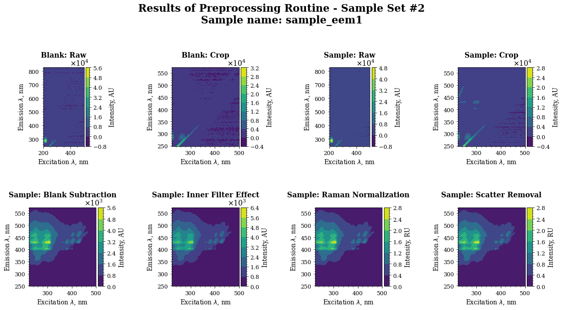
Visualize the preprocessing steps for a single sample
[11]:
import matplotlib.pyplot as plt
import matplotlib

sample_set = 2
sample_name = "sample_eem1"
axes = pyeem.plots.preprocessing_routine_plot(
    dataset,
    routine_results_df,
    sample_set=sample_set,
    sample_name=sample_name,
    plot_type="contour",
)
plt.show()
Load the calibration information
[12]:
cal_df = pyeem.preprocessing.calibration(
    dataset,
    routine_results_df
)
display(cal_df)
| concentration | integrated_intensity | prototypical_sample | hdf_path | |||||||
|---|---|---|---|---|---|---|---|---|---|---|
| source | source_units | intensity_units | measurement_units | slope | intercept | r_squared | ||||
| cigarette | ug/ml | Intensity, RU | Integrated Intensity, RU | 2533.174674 | -620.587879 | 0.929983 | 5.00 | 9937.219073 | True | preprocessing/complete/1/sample_eem2 |
| 0.929983 | 0.77 | 1598.421018 | False | preprocessing/complete/1/sample_eem3 | ||||||
| 0.929983 | 5.00 | 11369.642711 | True | preprocessing/complete/1/sample_eem6 | ||||||
| 0.929983 | 5.00 | 14786.022223 | False | preprocessing/complete/7/sample_eem1 | ||||||
| 0.929983 | 5.00 | 14005.964492 | False | preprocessing/complete/9/sample_eem1 | ||||||
| ... | ... | ... | ... | ... | ... | ... | ... | ... | ... | ... |
| wood_smoke | ug/ml | Intensity, RU | Integrated Intensity, RU | 4863.773278 | -1584.949118 | 0.460458 | 2.00 | 3387.998718 | False | preprocessing/complete/15/sample_eem16 |
| 0.460458 | 2.00 | 10022.795882 | False | preprocessing/complete/15/sample_eem6 | ||||||
| 0.460458 | 1.00 | 5014.273195 | False | preprocessing/complete/15/sample_eem5 | ||||||
| 0.460458 | 0.50 | 2636.485337 | False | preprocessing/complete/15/sample_eem4 | ||||||
| 0.460458 | 5.00 | 23200.187472 | True | preprocessing/complete/16/sample_eem1 |
81 rows × 4 columns
Checkout the calibration summary information
[13]:
cal_summary_df = pyeem.preprocessing.calibration_summary_info(cal_df)
display(cal_summary_df)
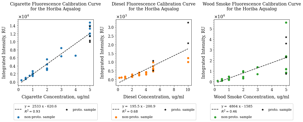
| source | source_units | intensity_units | measurement_units | slope | intercept | r_squared | Number of Samples | Min. Concentration | Max. Concentration | |
|---|---|---|---|---|---|---|---|---|---|---|
| 0 | cigarette | ug/ml | Intensity, RU | Integrated Intensity, RU | 2533.174674 | -620.587879 | 0.929983 | 26.0 | 0.2 | 5.0 |
| 1 | diesel | ug/ml | Intensity, RU | Integrated Intensity, RU | 195.502414 | -200.917295 | 0.684411 | 29.0 | 0.2 | 10.0 |
| 2 | wood_smoke | ug/ml | Intensity, RU | Integrated Intensity, RU | 4863.773278 | -1584.949118 | 0.460458 | 26.0 | 0.2 | 5.0 |
Plot the calibration curves
[14]:
axes = pyeem.plots.calibration_curves_plot(dataset, cal_df)
plt.show()
Create prototypical spectra and then plot them
[ ]:
proto_results_df = pyeem.augmentation.create_prototypical_spectra(
    dataset,
    cal_df
)
display(proto_results_df)

axes = pyeem.plots.prototypical_spectra_plot(
    dataset,
    proto_results_df,
    plot_type="contour"
)
plt.show()
Augmented Spectra - Single Sources
Create augmented single source spectra by scaling each prototypical spectrum across a range of concentrations
[ ]:
ss_results_df = pyeem.augmentation.create_single_source_spectra(
    dataset,
    cal_df,
    conc_range=(0, 5),
    num_spectra=1000
)
display(ss_results_df)
Plot the augmented single source spectra
[ ]:
from IPython.display import HTML
%matplotlib inline

source = "wood_smoke"
anim = pyeem.plots.single_source_animation(
    dataset,
    ss_results_df.iloc[::100, :],
    source=source,
    plot_type="imshow",
    fig_kws={"dpi": 120},
    animate_kws={"interval": 100, "blit": True},
)
HTML(anim.to_html5_video())
[ ]:
source = "diesel"
anim = pyeem.plots.single_source_animation(
    dataset,
    ss_results_df.iloc[::100, :],
    source=source,
    plot_type="imshow",
    fig_kws={"dpi": 120},
    animate_kws={"interval": 100, "blit": True},
)
HTML(anim.to_html5_video())
[ ]:
source = "cigarette"
anim = pyeem.plots.single_source_animation(
    dataset,
    ss_results_df.iloc[::100, :],
    source=source,
    plot_type="imshow",
    fig_kws={"dpi": 120},
    animate_kws={"interval": 100, "blit": True},
)
HTML(anim.to_html5_video())
Augmented Spectra - Mixtures
Create augmented mixture spectra by scaling and combining the prototypical spectra across a range of concentrations
[ ]:
mix_results_df = pyeem.augmentation.create_mixture_spectra(
    dataset,
    cal_df,
    conc_range=(0.01, 6.3),
    num_steps=15
)
display(mix_results_df)
Plot the augmented mixture spectra
[ ]:
anim = pyeem.plots.mixture_animation(
    dataset,
    mix_results_df.iloc[::100, :],
    plot_type="contour",
    fig_kws={"dpi": 100},
    animate_kws={"interval": 100, "blit": True},
)
HTML(anim.to_html5_video())
[ ]:
rutherfordnet = pyeem.analysis.models.RutherfordNet()
rutherfordnet.model.summary()
[ ]:
(x_train, y_train), (x_test, y_test) = rutherfordnet.prepare_data(
    dataset,
    ss_results_df,
    mix_results_df,
    routine_results_df
)
[ ]:
history = rutherfordnet.train(
    x_train,
    y_train
)
[ ]:
axes = pyeem.plots.model_history_plot(history)
plt.show()
[ ]:
train_predictions = rutherfordnet.model.predict(x_train)
test_predictions = rutherfordnet.model.predict(x_test)

train_pred_results_df = rutherfordnet.get_prediction_results(
    dataset,
    train_predictions,
    y_train
)

test_pred_results_df = rutherfordnet.get_prediction_results(
    dataset,
    test_predictions,
    y_test
)

axes = pyeem.plots.prediction_parity_plot(
    dataset,
    test_pred_results_df,
    train_df=train_pred_results_df
)
plt.show()
[ ]: