Tutorial #2 - Preprocessing options
Check out the supported instruments
[2]:
pyeem.instruments.supported
[2]:
| name | ||
|---|---|---|
| manufacturer | supported_models | |
| Agilent | Cary 4E | cary_4e |
| Cary Eclipse | cary_eclipse | |
| Horiba | Aqualog-880-C | aqualog |
| SPEX Fluorolog-3 | fluorolog | |
| Tecan | Spark | spark |
Check out the demo datasets
[3]:
demos_df = pyeem.datasets.demos
display(demos_df)

print("Dataset description for the drEEM demo:")
print(demos_df[
    demos_df["demo_name"] == "drEEM"
]["description"].item())
| demo_name | description | citation | DOI | absorbance_instrument | water_raman_instrument | EEM_instrument | |
|---|---|---|---|---|---|---|---|
| 0 | rutherford | Excitation Emission Matrix (EEM) fluorescence ... | Rutherford, Jay W., et al. "Excitation emissio... | 10.1016/j.atmosenv.2019.117065 | Aqualog | None | Aqualog |
| 1 | drEEM | The demo dataset contains measurements made du... | Murphy, Kathleen R., et al. "Fluorescence spec... | 10.1039/c3ay41160e | Cary 4E | Fluorolog | Fluorolog |
Dataset description for the drEEM demo:
The demo dataset contains measurements made during four surveys of San Francisco Bay that took place in spring, summer, autumn and winter 2006 (Murphy et al. 2013, J. Mar. Syst. 111-112, 157-166).
Download the drEEM demo dataset from S3
Please note that this step requires an internet connection because the data is downloaded from an AWS S3 bucket.
[4]:
demo_data_dir = pyeem.datasets.download_demo(
    "demo_data",
    demo_name="drEEM"
)
Download Demo Dataset from S3: 100%|██████████| 260/260 [00:00<00:00, 163031.70it/s]
Load the dataset
[5]:
demo_data_dir = "demo_data/drEEM"

dataset = pyeem.datasets.Dataset(
    data_dir=demo_data_dir,
    raman_instrument="fluorolog",
    absorbance_instrument="cary_4e",
    eem_instrument="fluorolog",
    mode="w"
)
WARNING: No Sample EEM scans were found in sample set 1.
WARNING: No corresponding absorbance scan for sample EEM sample_eem2.csv in sample set 8. There should be an absorbance measurement named absorb2.csv in this sample set.
Let’s checkout the metadata
The metadata contains information about collected sample sets which are composed of a few different scan types.
[6]:
display(dataset.meta_df)
| datetime_utc | filename | collected_by | description | comments | water_raman_wavelength | dilution_factor | cruise | Site | Rep | SampID | filepath | name | hdf_path | ||
|---|---|---|---|---|---|---|---|---|---|---|---|---|---|---|---|
| sample_set | scan_type | ||||||||||||||
| 1 | water_raman | 2006-04-27 00:00:00 | water_raman1.csv | Anon | 275.0 | 1.0 | SF-p-win | 1B | 3.0 | 478.0 | /home/roboat/Documents/roboat/PyEEM/docs/sourc... | water_raman1 | raw_sample_sets/1/water_raman1 | ||
| blank_eem | 2006-04-27 11:59:30 | blank_eem1.csv | Anon | NaN | 1.0 | SF-p-win | 1B | 3.0 | 478.0 | /home/roboat/Documents/roboat/PyEEM/docs/sourc... | blank_eem1 | raw_sample_sets/1/blank_eem1 | |||
| absorb | 2006-04-27 23:59:00 | absorb1.csv | Anon | NaN | 1.0 | SF-p-win | 1B | 3.0 | 478.0 | /home/roboat/Documents/roboat/PyEEM/docs/sourc... | absorb1 | raw_sample_sets/1/absorb1 | |||
| 2 | water_raman | 2006-04-28 00:00:00 | water_raman1.csv | Anon | 275.0 | 1.0 | SF-p-win | 1B | 2.0 | 477.0 | /home/roboat/Documents/roboat/PyEEM/docs/sourc... | water_raman1 | raw_sample_sets/2/water_raman1 | ||
| blank_eem | 2006-04-28 05:59:45 | blank_eem1.csv | Anon | NaN | 1.0 | SF-p-win | 1B | 2.0 | 477.0 | /home/roboat/Documents/roboat/PyEEM/docs/sourc... | blank_eem1 | raw_sample_sets/2/blank_eem1 | |||
| ... | ... | ... | ... | ... | ... | ... | ... | ... | ... | ... | ... | ... | ... | ... | ... |
| 15 | absorb | 2006-09-14 23:59:00 | absorb11.csv | Anon | NaN | 1.0 | SF-p-win | 3A | 3.0 | 493.0 | /home/roboat/Documents/roboat/PyEEM/docs/sourc... | absorb11 | raw_sample_sets/15/absorb11 | ||
| 16 | water_raman | 2006-09-15 00:00:00 | water_raman1.csv | Anon | 275.0 | 1.0 | SF-p-win | 3A | 1.0 | 491.0 | /home/roboat/Documents/roboat/PyEEM/docs/sourc... | water_raman1 | raw_sample_sets/16/water_raman1 | ||
| blank_eem | 2006-09-15 07:59:40 | blank_eem1.csv | Anon | NaN | 1.0 | SF-p-win | 3A | 1.0 | 491.0 | /home/roboat/Documents/roboat/PyEEM/docs/sourc... | blank_eem1 | raw_sample_sets/16/blank_eem1 | |||
| sample_eem | 2006-09-15 15:59:20 | sample_eem1.csv | Anon | NaN | 1.0 | SF-p-win | 3A | 1.0 | 491.0 | /home/roboat/Documents/roboat/PyEEM/docs/sourc... | sample_eem1 | raw_sample_sets/16/sample_eem1 | |||
| absorb | 2006-09-15 23:59:00 | absorb1.csv | Anon | NaN | 1.0 | SF-p-win | 3A | 1.0 | 491.0 | /home/roboat/Documents/roboat/PyEEM/docs/sourc... | absorb1 | raw_sample_sets/16/absorb1 |
182 rows × 14 columns
Checkout the metadata summary information
[7]:
dataset.metadata_summary_info()
[7]:
| Start datetime (UTC) | End datetime (UTC) | Number of sample sets | Number of blank EEMs | Number of sample EEMs | Number of water raman scans | Number of absorbance scans | |
|---|---|---|---|---|---|---|---|
| 0 | 2006-04-27 | 2006-09-15 23:59:00 | 16 | 16 | 73 | 16 | 77 |
[8]:
from IPython.display import HTML
fig_kws = {"dpi": 200}
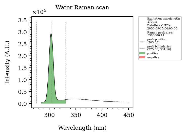
anim = pyeem.plots.water_raman_peak_animation(dataset, excitation_wavelength=275, fig_kws=fig_kws)
HTML(anim.to_html5_video())
[8]:
[9]:
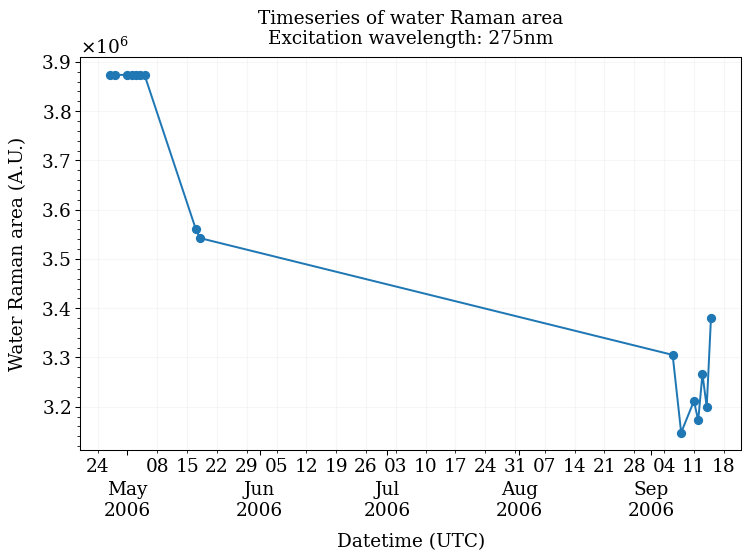
import matplotlib.pyplot as plt
fig_kws={"dpi": 95}
plot_kws = {"fmt": "o-"}
kwargs = {"byweekday": 0}
ax = pyeem.plots.water_raman_timeseries(
    dataset,
    excitation_wavelength=275,
    fig_kws=fig_kws,
    plot_kws=plot_kws,
    **kwargs
)
plt.show()
Create a preprocessing routine
The demo dataset contains raw scans, in order to analyze and interpret this data, we must first apply several preprocessing steps.
[10]:
routine_df = pyeem.preprocessing.create_routine(
    crop = False,
    discrete_wavelengths = False,
    gaussian_smoothing = False,
    blank_subtraction = True,
    inner_filter_effect = True,
    raman_normalization = True,
    scatter_removal = True,
    dilution = False,
)

display(routine_df)
| step_name | hdf_path | |
|---|---|---|
| step_order | ||
| 0 | raw | raw_sample_sets/ |
| 1 | blank_subtraction | preprocessing/corrections/blank_subtraction |
| 2 | inner_filter_effect | preprocessing/corrections/inner_filter_effect |
| 3 | raman_normalization | preprocessing/corrections/raman_normalization |
| 4 | scatter_removal | preprocessing/corrections/scatter_removal |
| 5 | complete | preprocessing/complete/ |
Execute the preprocessing routine
Each preprocessing step has certain knobs and dials you can tune to have them run to your liking. It is worth checking the documentation to learn more about these customizations.
Please note that depending on the steps and settings you’ve chosen as well as your dataset’s size, the time it takes for this step to complete will vary.
[11]:
kwargs = {
    "raman_source_type": "water_raman",
    "water_raman_wavelength": 275,
    "excision_width": 30,
    "fill": "interp",
}


routine_results_df = pyeem.preprocessing.perform_routine(
    dataset,
    routine_df,
    progress_bar=True,
    **kwargs
)

display(routine_results_df)
Preprocessing scan sets: 100%|██████████| 16/16 [00:38<00:00, 2.43s/it]
| step_completed | step_exception | hdf_path | units | ||||
|---|---|---|---|---|---|---|---|
| sample_set | scan_type | name | step_name | ||||
| 1 | blank_eem | blank_eem1 | raw | True | None | raw_sample_sets/1/blank_eem1 | Intensity, AU |
| 2 | blank_eem | blank_eem1 | raw | True | None | raw_sample_sets/2/blank_eem1 | Intensity, AU |
| sample_eem | sample_eem1 | raw | True | None | raw_sample_sets/2/sample_eem1 | Intensity, AU | |
| blank_subtraction | True | None | preprocessing/corrections/blank_subtraction/2/... | Intensity, AU | |||
| inner_filter_effect | True | None | preprocessing/corrections/inner_filter_effect/... | Intensity, AU | |||
| ... | ... | ... | ... | ... | ... | ... | ... |
| 16 | sample_eem | sample_eem1 | blank_subtraction | True | None | preprocessing/corrections/blank_subtraction/16... | Intensity, AU |
| inner_filter_effect | True | None | preprocessing/corrections/inner_filter_effect/... | Intensity, AU | |||
| raman_normalization | True | None | preprocessing/corrections/raman_normalization/... | Intensity, RU | |||
| scatter_removal | True | None | preprocessing/corrections/scatter_removal/16/s... | Intensity, RU | |||
| complete | True | None | preprocessing/complete/16/sample_eem1 | Intensity, RU |
454 rows × 4 columns
Check to see if any of the steps failed to complete
If you are using a demo dataset, you should see an empty dataframe.
[12]:
display(routine_results_df[
    routine_results_df["step_exception"].notna()
])
| step_completed | step_exception | hdf_path | units | ||||
|---|---|---|---|---|---|---|---|
| sample_set | scan_type | name | step_name | ||||
| 8 | sample_eem | sample_eem2 | inner_filter_effect | False | 'No object named raw_sample_sets/8/absorb2 in ... | None | None |
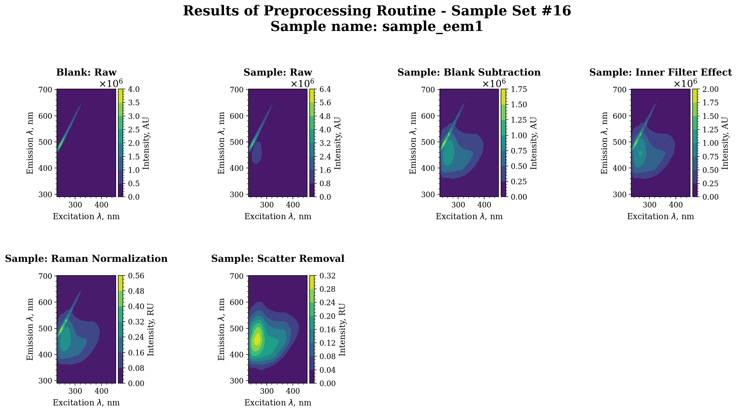
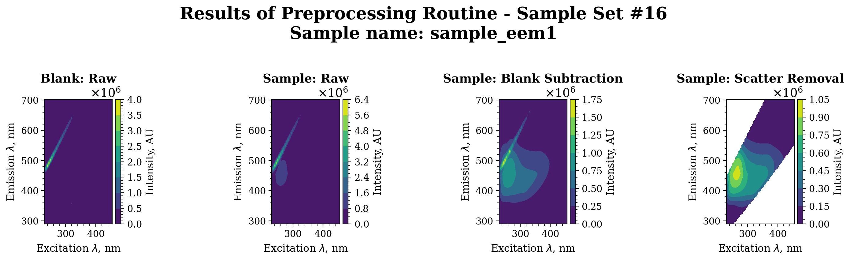
Visualize the preprocessing steps for a single sample
[13]:
import matplotlib.pyplot as plt

sample_set = 16
sample_name = "sample_eem1"
axes = pyeem.plots.preprocessing_routine_plot(
    dataset,
    routine_results_df,
    sample_set=sample_set,
    sample_name=sample_name,
    plot_type="contour",
    fig_kws={"dpi": 200},
)
plt.show()
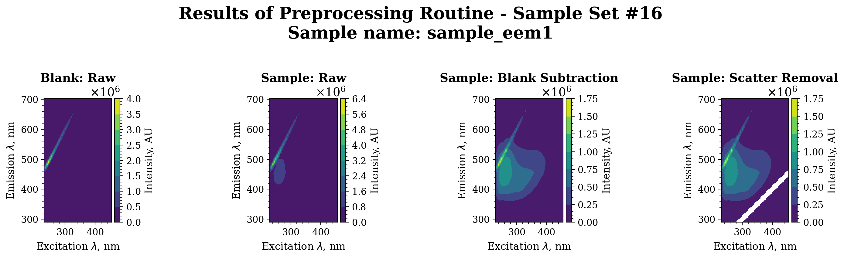
[14]:
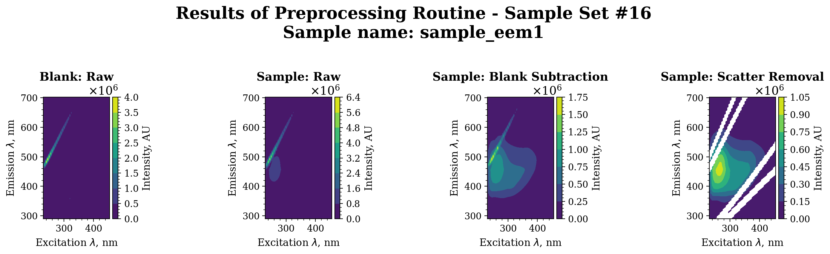
routine_df = pyeem.preprocessing.create_routine(
    crop = False,
    discrete_wavelengths = False,
    gaussian_smoothing = False,
    blank_subtraction = True,
    inner_filter_effect = False,
    raman_normalization = False,
    scatter_removal = True,
    dilution = False,
)

display(routine_df)
| step_name | hdf_path | |
|---|---|---|
| step_order | ||
| 0 | raw | raw_sample_sets/ |
| 1 | blank_subtraction | preprocessing/corrections/blank_subtraction |
| 2 | scatter_removal | preprocessing/corrections/scatter_removal |
| 3 | complete | preprocessing/complete/ |
[15]:
routine_results_df = pyeem.preprocessing.perform_routine(
    dataset,
    routine_df,
    fill = None,
    excision_width = 25,
    progress_bar=True
)

axes = pyeem.plots.preprocessing_routine_plot(
    dataset,
    routine_results_df,
    sample_set=sample_set,
    sample_name=sample_name,
    plot_type="contour",
    fig_kws={"dpi": 200},
)
plt.show()
Preprocessing scan sets: 100%|██████████| 16/16 [00:03<00:00, 4.09it/s]
[16]:
routine_results_df = pyeem.preprocessing.perform_routine(
    dataset,
    routine_df,
    raman_source_type = "water_raman",
    fill = None,
    truncate = "both",
    progress_bar=True
)

axes = pyeem.plots.preprocessing_routine_plot(
    dataset,
    routine_results_df,
    sample_set=sample_set,
    sample_name=sample_name,
    plot_type="contour",
    fig_kws={"dpi": 200},
)
plt.show()
Preprocessing scan sets: 100%|██████████| 16/16 [00:03<00:00, 4.21it/s]
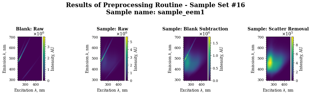
[17]:
routine_results_df = pyeem.preprocessing.perform_routine(
    dataset,
    routine_df,
    raman_source_type = "water_raman",
    fill = None,
    band="rayleigh",
    order="first",
    excision_width=20,
    progress_bar=True
)

axes = pyeem.plots.preprocessing_routine_plot(
    dataset,
    routine_results_df,
    sample_set=sample_set,
    sample_name=sample_name,
    plot_type="contour",
    fig_kws={"dpi": 200},
)
plt.show()
Preprocessing scan sets: 100%|██████████| 16/16 [00:03<00:00, 4.09it/s]
[18]:
routine_results_df = pyeem.preprocessing.perform_routine(
    dataset,
    routine_df,
    raman_source_type = "water_raman",
    fill = "interp",
    band="both",
    excision_width = 25,
    progress_bar=True
)

axes = pyeem.plots.preprocessing_routine_plot(
    dataset,
    routine_results_df,
    sample_set=sample_set,
    sample_name=sample_name,
    plot_type="imshow",
)
plt.show()
Preprocessing scan sets: 100%|██████████| 16/16 [00:08<00:00, 1.97it/s]
[ ]:
routine_results_df = pyeem.preprocessing.perform_routine(
    dataset,
    routine_df,
    raman_source_type = "water_raman",
    fill = None,
    band="rayleigh",
    order="first",
    truncate="below",
    excision_width = 25,
    progress_bar=True
)

axes = pyeem.plots.preprocessing_routine_plot(
    dataset,
    routine_results_df,
    sample_set=sample_set,
    sample_name=sample_name,
    plot_type="imshow",
)
plt.show()
[ ]: